Design Explanations¶

Some of the implementations of the subroutines in Workbench Algorithms have non-trivial implementation details (from a classical software perspective) that users may want further elaboration on. The pages indexed here provide explanations for these aspects and justifications for the choices made in their design. This is purely to provide some background information and elaboration on design decisions -- the pages here are not designed to teach users how to use the software in their own work. For example implementations that can help with this, see the Tutorials pages.

What is generalized multiplexing?¶

Multiplexing is a quantum operation that can be thought of as the quantum equivalent of a classical for loop. It is typically written as

\[ \sum_{i=0}^{d-1} |i\rangle\langle i| \otimes U_i \ , \]

where \(U_i\) is some unitary operator indexed by \(i\). In the generalized multiplexing framework as implemented in Workbench Algorithms, we modify this slightly to introduce a function of the index \(i\):

\[ \sum_{i=0}^{d-1} |i\rangle\langle i| \otimes F(i) \ , \]

where \(F(i)^\dagger F(i) = \mathbb{I}\) for all \(i\). We can think about this in classical programming terms as implementing a series of if statements inside the for loop (for those familiar with C++, the implementation is actually more like switch/case, but for consistency we will stick with python):

for i in range(d):
    if i == 0:
        # do something
    elif i == 1:
        # do something different
    ...
    # etc

The function \(F(i)\) provides the means for doing these "somethings" and in generalized multiplexing, we do not make any restrictions on what may be done as part of the definition of \(F\) (aside from the unitarity constraint mentioned above).

The two aspects of multiplexing and separation of concerns¶

There are two aspects of generalized multiplexing that each require separate machinery to implement:

The machinery to implement the indexing \(\sum_{i=0}^{d-1} |i\rangle\langle i|\) (i.e. the for loop operation).
The machinery to implement \(F(i)\) (i.e. the if statement operations).

These can be clearly seen with reference to Fig. 2 in the Even more efficient quantum computations of chemistry through tensor hypercontraction paper:

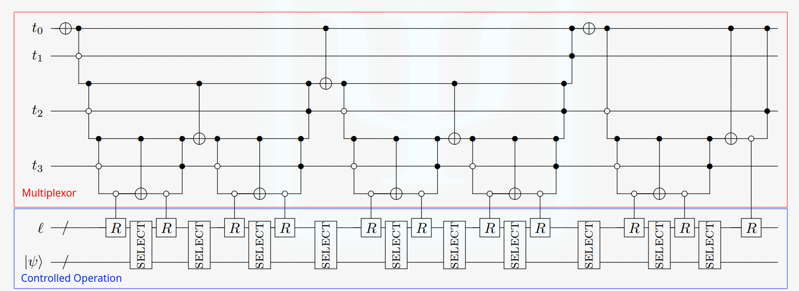
The top part of the circuit (shown in red and labelled "Multiplexor") is an efficient method to implement the for loop while the bottom part (shown in blue and labelled "Controlled operation") realizes the if statement operations (explicitly, we could think of this particular example as saying "if i == d-1, apply \(R\), else apply \(R\) followed by \(\text{SELECT}\)).

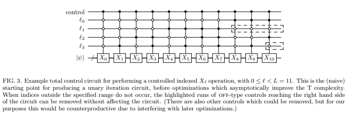
These two concerns are entirely separable, and we should be able to treat them independently -- e.g. if someone comes up with a more efficient multiplexor, then we should be able to swap that out in a code implementation of the above circuit without touching the code for the controlled operations. In fact, we already have reason to do this: while the above is the most gate-efficient method we currently have, it is not particularly intuitive to look at, nor is it particularly sim-efficient. When debugging and developing code, it is more convenient to use a less gate efficient but more straightforward implementation like Fig. 3 in the Encoding Electronic Spectra in Quantum Circuits with Linear T Complexity paper ⧉:

In Workbench Algorithms, these two aspects are split up into two separate objects: Multiplexor Qubricks and multiplexing functions.

`Multiplexor` `Qubricks`¶

Conceptually, these Qubricks are relatively straightforward, and so we won't dwell on them for too long here. The role of these Qubricks is to perform the quantum for loop, for which it needs three inputs:

The Qubits register over which to apply the control structure.
A list of indices that the control terms are applied on.
A (classical) multiplexing function that implements the controlled operation.

All three of these are passed at the Qubrick compute.

The first is straightforward: the Qubrick needs some qubits on which it can perform the operations.

The second essentially informs the Qubrick about whether it needs to skip any indices; for some multiplexors, this will involve skipping more than just the controlled operation, and so this needs to be passed to it.

The structure of the third operation will be elaborated in the following section, but for now, consider what inputs the multiplexing function actually needs: it needs to know what index the for loop is currently on so it can generate \(F(i)\) appropriately; it needs a Qubits object that the operation can be controlled on; finally, it needs any "meta-control" qubits that the entire multiplexing operation is controlled on (see the qubit labelled "control" above). Every multiplexed operation needs access to these three inputs -- in the Workbench Algorithms implementation this is all of the inputs that the multiplexing functions are allowed to have!

We will elaborate on how one can have fully general functions with such a limited number of inputs in the following section.

Multiplexing functions and the factory pattern¶

Let's return to the fundamental equation for generalized multiplexing to ground ourselves:

\[ \sum_{i=0}^{d-1} |i\rangle\langle i| \otimes F(i) \ , \]

Ignoring the "meta-control" qubit (as it is not really relevant to our discussion here), it should be fairly clear that our function \(F(i)\) really should only take in a (classical) index \(i\) such that we can generate \(F(i)\) and a Qubits object that allows us to control \(F(i)\) properly.

But if we want to do arbitrary operations, we will inevitably end up with a whole bunch of additional arguments that are needed to specify the operation we want! How do we handle this?

To illustrate the implementation (and to show that this is a real concern, not simply something abstract that we don't need to worry about), let's return to the example from the THC paper. Ignoring the multiplexor part (since we've separated out that concern), we could write a first pass for the multiplexing function as:

def thc_multiplexing_func(index, index_reg, ell_reg, psi_reg, num_terms, R, Select, ctrl=0):
    if index == num_terms - 1:
        R.compute(ell_reg, index_reg | ctrl)
    else:
        R.compute(ell_reg, index_reg | ctrl)
        Select.compute(ell_reg, psi_reg)

Despite the fact that this is a pretty straightforward multiplexed operation, we've already ballooned out to 8 inputs! As the multiplexed operations get more complicated, the signatures of the multiplexing functions will also get more complicated, exacerbating the situation even further.

Instead of passing this function (and all its arguments) down throughout the Qubrick, we can use the factory pattern to generate a far more useable function by tying down all the unnecessary parameters.

The factory pattern¶

In software design, a factory is a function that returns some object (either another function or a class). It can be used to enforce some interface structure from disparate data. The general pattern looks like this:

def generic_factory(<some args>):
    <some pre-processing>
    def output_function(<other args>):
        ...
    return output_function

This will be clearer if we return to the THC example above. Let's say we want to write a Qubrick for the circuit:

class THCMultiplexing(Qubrick):
    def __init__(self, multiplexor):
        super().__init__()
        self.multiplexor = multiplexor

Since we've separated out our multiplexor, we can pass this in the __init__ and we no longer have to worry about it. All we need to worry about is the multiplexing function, which we need to define in the _compute method (since it requires Qubits registers):

class THCMultiplexing(Qubrick):
    def __init__(self, multiplexor, R, Select):
        super().__init__()
        self.multiplexor = multiplexor
        self.R = R
        self.Select = Select

    def _compute(self, index_reg, ell_reg, psi_reg, num_terms, ctrl=0):
        multiplexing_function = self.thc_multiplexing_factory(ell_reg, psi_reg, num_terms)
        used_indices = [1] * num_terms
        self.multiplexor.compute(index_reg, multiplexing_function, used_indices, ctrl=ctrl)

    def thc_multiplexing_factory(self, ell_reg, psi_reg, num_terms):
        def thc_multiplexing_func(index, index_reg, ctrl=0):
            if index == num_terms - 1:
                self.R.compute(ell_reg, index_reg | ctrl)
            else:
                self.R.compute(ell_reg, index_reg | ctrl)
                self.Select.compute(ell_reg, psi_reg)
        return thc_multiplexing_func

This is the full Qubrick that we can now use to do multiplexing. Let's break down all the aspects:

The R and Select Qubricks are now in the __init__, so they don't have to be explicitly passed anymore.
We've defined a new thc_multiplexing_factory method which generates our multiplexing function. It takes in the Qubits registers that the controlled operations act on (not the index_reg though -- this is passed when the function is executed) and the classical num_terms parameter.

This effectively "freezes out" these parameters so that the actual multiplexing function (which is returned from the factory as thc_multiplexing_func) only takes in the arguments that are necessary for all multiplexors. One can think of the factory as generating \(F(i)\) so that it can be passed to the multiplexor.
In this particular case, we're not skipping any indices, so all of the indices are used.
We can then compute the multiplexor, which has no idea any of the ell_reg, psi_reg etc exist, it just does the for loop in exactly the same way is would for any other operation.

Conclusion¶

Generalized multiplexing is an incredibly powerful tool that can allow us to implement effectively arbitrary operations, but that doesn't mean there is no structure to it. We showed how we can separate out the concerns of the multiplexor and the controlled operation so that we can swap different implementations out to our heart's content. We also argued that the multiplexing function \(F(i)\), in acting as a quantum if statement really should only take in the classical index \(i\) and the control register as inputs. We showed how by using factories we can generate such \(F(i)\) functions from more general functions by freezing out additional parameters.